
Beyond Static Timeouts: Smarter Deadman Alerts Using Beta-Bernoulli Modeling
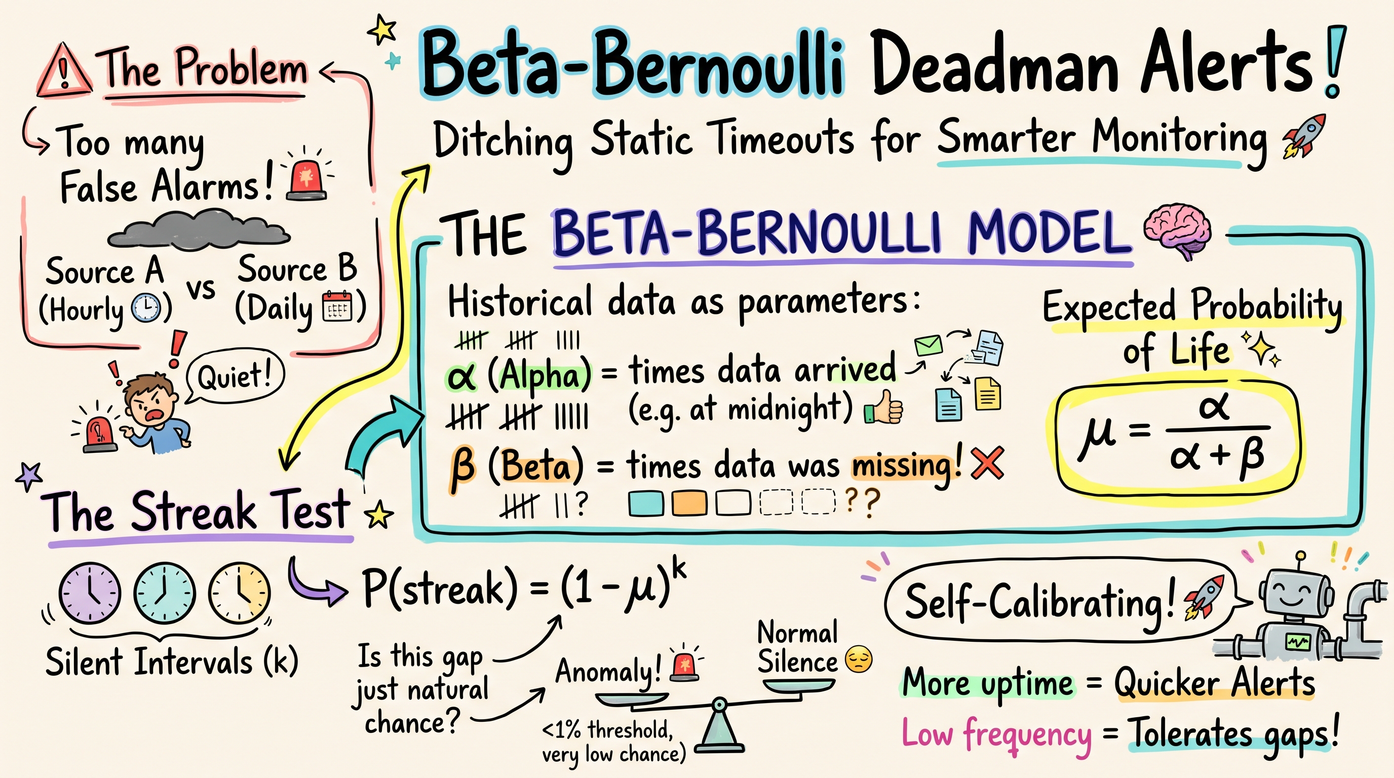
Monitoring automated data pipelines, IoT telemetry, and scheduled batch integrations often leads to an operational nightmare: static timeout fatigue.
In real-world environments, not all sources behave identically:
- Source A pushes telemetry every hour without fail.
- Source B uploads a batch file only once every few days.
- Source C is an intermittent integration that routinely pauses during quiet windows.
If you set a hardcoded static alert rule like "Alert if no data arrives in 4 hours", Source B triggers constant false positives, while Source A could be down for three full hours before anyone notices.
Here is how a lightweight Bayesian concept—the Beta-Bernoulli model—solves this problem dynamically.
The Problem with Static Thresholds
Static thresholds force engineering teams into an uncomfortable compromise between two failure modes:
- Alert Flooding: Overly aggressive thresholds trigger false alarms for naturally intermittent data producers.
- Delayed Incident Detection: Overly permissive thresholds delay detection when high-frequency critical producers silently stall.
Maintaining custom timeout configurations across hundreds of integrations does not scale. What you need is an alert mechanism that adapts to each integration's historical arrival pattern.
How It Works: The Intuition
Instead of hardcoding hours or days, we track two counts for each integration over regular observation intervals:
- (Alpha): The number of intervals where data arrived as expected.
- (Beta): The number of intervals where no data arrived.
The interval unit can be anything you choose—a day, an hour, or five minutes—as long as it matches your sampling window.
1. Estimating Baseline Inactivity
The expected probability of seeing activity in any given interval is:
Consequently, the expected probability that an interval is silent is:
2. Evaluating the Silence Streak
When a pipeline goes quiet for consecutive intervals, we ask:
"What is the probability of seeing a gap this long purely by chance?"
Assuming intervals are independent, the probability of consecutive silent intervals is:
If this probability drops below a chosen significance threshold (e.g., ), we declare the silence an anomaly and trigger an alert.
Why This Works So Well in Production
- Self-Calibrating: High-reliability producers (e.g., ) trigger alerts after just 2 silent intervals. Intermittent producers (e.g., ) naturally require a much longer gap before an alert fires.
- Unit Agnostic: The math does not care whether your interval represents hours, days, or heartbeat pings.
- Low Overhead: You only store two numbers ( and ) per integration. No complex machine learning models, training pipelines, or expensive time-series databases required.
- Simple Developer Interface: Downstream alerting services only consume a clean boolean (
True/False), leaving the statistical complexity encapsulated within the monitoring helper.
By switching from arbitrary static timeouts to streak probabilities, you drastically reduce alarm fatigue while catching actual outages significantly faster.